
How to Parse and Visualize Strava Activities with Python and Matplotlib - Awesome Strava Charts #1
Download and parse Strava GPX files and visualize activity coordinates with a scatter plot.

Strava charts give you basic insights into your workout, but that’s about it.
Even in the premium plan, the amount of analytics you can dive into is limited. But here’s a silver lining - if you have basic programming skills, you can create your own analyses and visualizations in a matter of minutes.
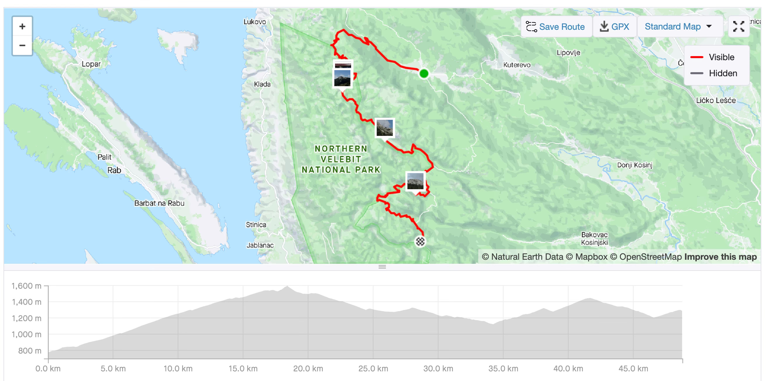
You can download a GPX file from any Strava workout through its web app. I’ll use one of my recent mountain bike rides through Velebit National Park in Croatia. The ride is almost 50 kilometers long and has more than 1400 meters of elevation gain:
You can download any of your workouts to follow along, or just download mine from GitHub.
This article is the first one in the series and will focus mostly on reading and parsing GPX files in Python. There’s one visualization at the end, but fear not, many more are coming in the future.

If you’re a paid subscriber, you can download the data and the notebook on the GitHub repo.
Let’s dig in!
How to Read GPX Files in Python
You’ll need to install the gpxpy library to read GPX files with Python:
pip install gpxpyOnce installed, stick the following imports at the top of your notebook:
import gpxpy
import gpxpy.gpx
import pandas as pd
import matplotlib as mpl
import matplotlib.pyplot as plt
A GPX file is nothing more than an XML file with some specific data point names:

So, it’s a collection of points containing latitude, longitude, elevation, and time information, but also “hidden” details such as temperature and heart rate in the extensions.
Note that you might not have these fields if your GPS unit doesn’t record temperature or you aren’t wearing a heart rate monitor. On the other side, you might have some additional ones if you’re recording power and cadence.
GPX files are typically loaded through Python’s context manager syntax, followed by a call to gpxpy.parse() function on the raw file:
with open("../data/src_mtb_ride.gpx", "r") as gpx_file:
    gpx = gpxpy.parse(gpx_file)

gpx
As long as you see a GPXTracker object that has a segment of points, you’re good to go.
You can extract a couple of quick statistics from the loaded GPX file:
print(f"Number of track points: {gpx.get_track_points_no()}")
print(f"Duration in seconds:    {gpx.get_duration():.2f}")
print(f"Duration in hours:      {(gpx.get_duration() / 3600):.2f}")
print(f"Minimum elevation:      {gpx.get_elevation_extremes().minimum}")
print(f"Maximum elevation:      {gpx.get_elevation_extremes().maximum}")
print(f"Total uphill:           {gpx.get_uphill_downhill().uphill:.2f}")
print(f"Total downhill:         {gpx.get_uphill_downhill().downhill:.2f}")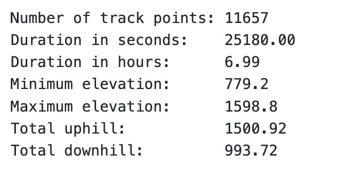
So, the file has over 11K data points and represents a ride that lasted almost 7 hours.
Every track point carries more valuable information, so let’s see how to extract them.
How to Parse GPX Data Points
If you call the get_points_data() function on the loaded GPX file, you’ll get a list of those 11K track points:
point_data = gpx.get_points_data()
point_data[10000:10010]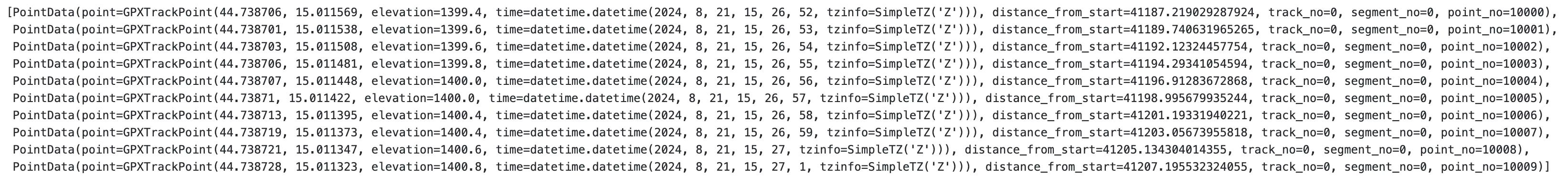
Every point has a geolocation, elevation in meters, timestamp when it was recorded, how far from the start it was recorded, and other, less relevant metadata fields.
You can access individual properties of a single track point with the following code:
p = point_data[10000]

print(f"Latitude:            {p.point.latitude}")
print(f"Longitude:           {p.point.longitude}")
print(f"Elevation:           {p.point.elevation}")
print(f"Distance from start: {p.distance_from_start}")
print(f"Time:                {p.point.time}")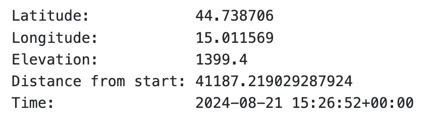
The extension data is hidden, and you’ll have to access it in an entirely different way:
point_extensions = [point.extensions[0] for point in gpx.tracks[0].segments[0].points]
point_extensions[10000:10010]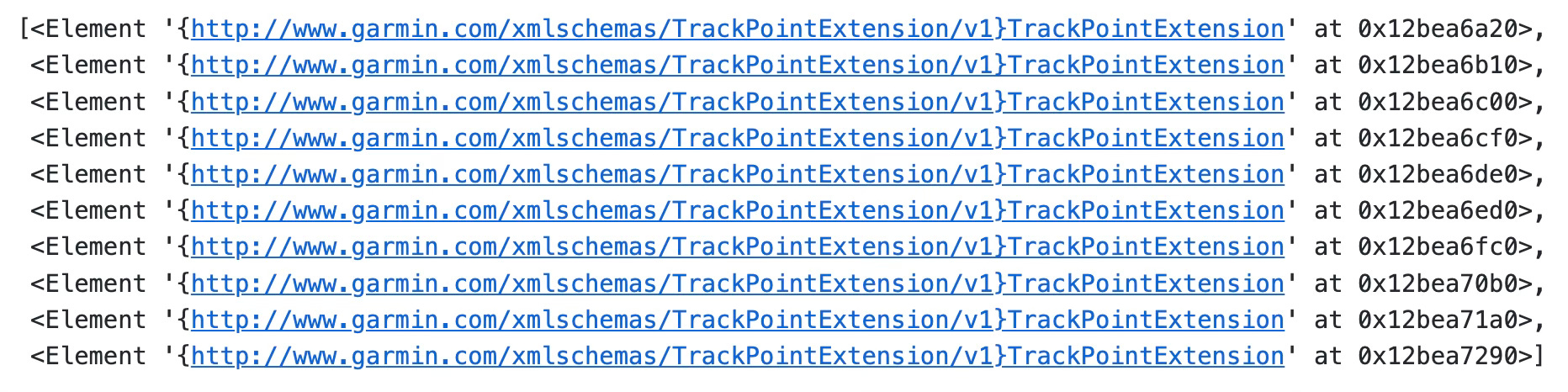
Each <Element> has properties tag and text you can extract. The first one represents the property name while the other is textual value:
for ext in point_extensions[10000]:
    print(ext.tag, ext.text)
You’ll have to perform some string manipulation and splitting to remove unwanted text from the extension tag:
for ext in point_extensions[10000]:
print(ext.tag.split("}")[-1], ext.text) 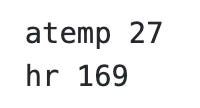
Next, let’s parse the whole thing!
Here’s what the following snippet does:
Iterates over all track points, starting from the second one
Calculates the time difference between track point T2 and track point T1
Calculates the distance in meters between T1 and T2
Gets the average speed in meters per second (m/s) and converts it to kilometers per hour (km/h)
Checks for possible errors in speed data - any speed above 15 m/s (54 km/h) is topped at that point (I’m slow)
Extract temperature and heart rate from the extensions list
data_parsed = []

for i in range(1, len(point_data)):
    # Previous and current points
    p1 = point_data[i - 1]
    p2 = point_data[i]

    # Calculate time difference in seconds
    time_diff = (p2.point.time - p1.point.time).total_seconds()
    # Don't consider points where time difference is 0 or less
    if time_diff <= 0:
        continue

    # Distance in meters
    distance_diff = p2.point.distance_2d(p1.point)

    # Speed in m/s (meters per second)
    speed_ms = p2.point.speed_between(p1.point)

    # Sanity check - I'm not that fast
    if speed_ms > 15:
        speed_ms = 15

    # Speed in km/h (kilometers per hour)
    speed_kmh = speed_ms * 3.6

    # Heart rate and temperature
    ext_data = []
    for ext in point_extensions[i - 1]:
        ext_data.append(ext.text)

    # Append
    data_parsed.append({
        "latitude": p2.point.latitude,
        "longitude": p2.point.longitude,
        "elevation": p2.point.elevation,
        "distance_from_start": p2.distance_from_start,
        "time_of_day": p2.point.time,
        "time_in_seconds_from_prev": time_diff,
        "distance_in_meters_from_prev": distance_diff,
        "speed_ms": speed_ms,
        "speed_kmh": speed_kmh,
        "temperature_c": int(ext_data[0]),
        "heart_rate": int(ext_data[1])
    })

data_parsed[5555]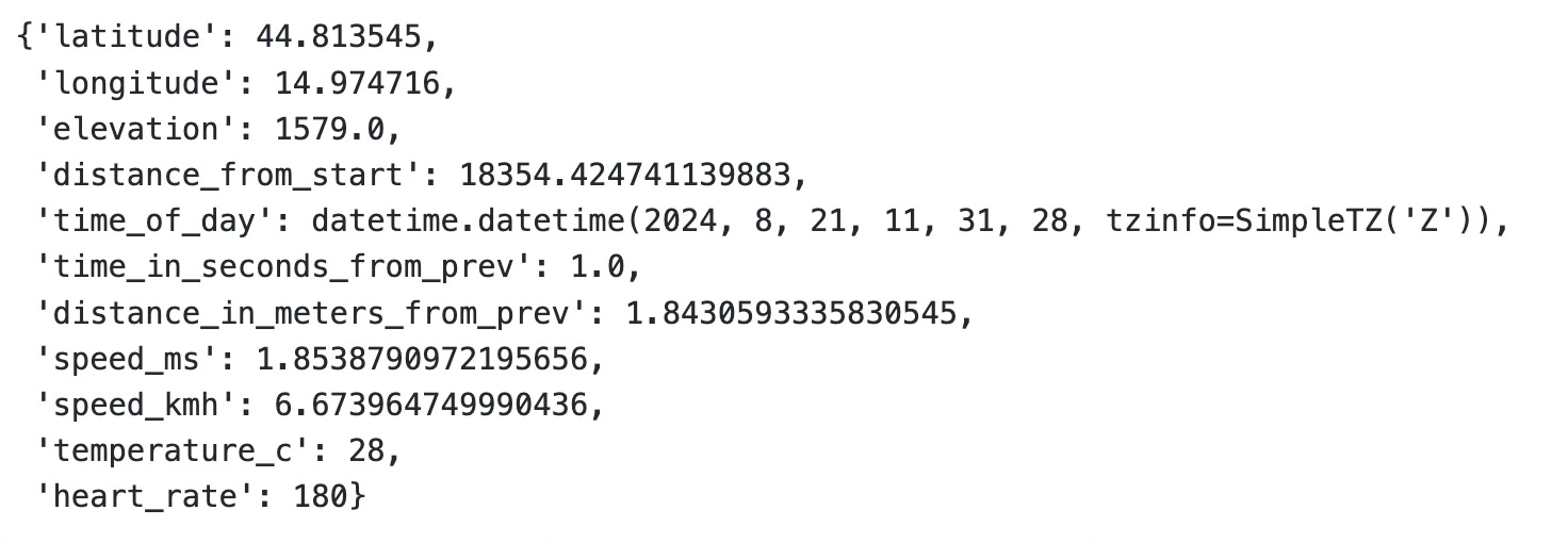
You now have much more detailed insights into the Strava activity.
Save this data to disk, as you’ll use it throughout the series. The code snippet below adds the row_id column so you can always sort the dataset if rows get out of order:
df = pd.DataFrame(data_parsed)
df.to_csv("strava_parsed.csv", index=True, index_label="row_id")
df.head(10)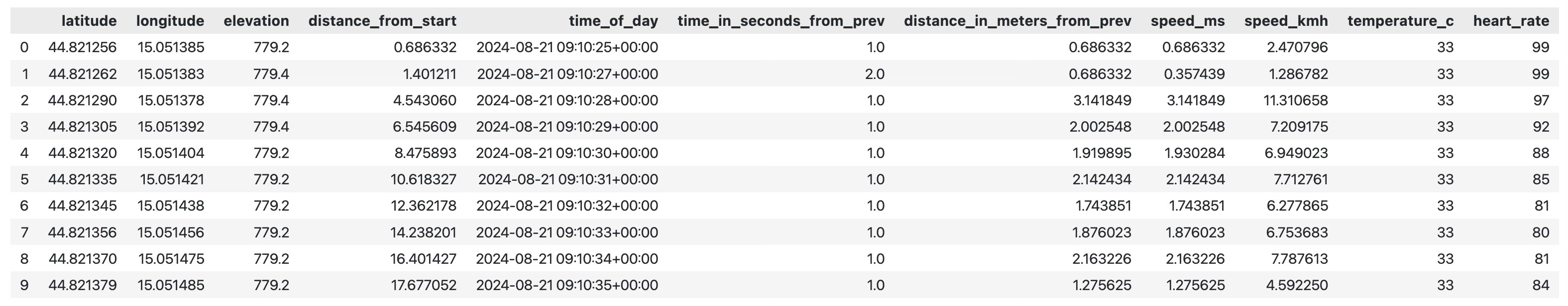
Visualize Strava Activity Route as a Scatter Plot Map
The latitude, longitude, and speed_kmh are the 3 columns you’ll need for visualization purposes.
Read this article to get my Matplotlib theme:
Matplotlib isn’t the best option for visualizing maps, but it’s great for showing scatter plots. That’s all an activity plot is, in a nutshell. The only thing you’ll be missing is the background, which is the map itself.
The plot should still resemble the original route.
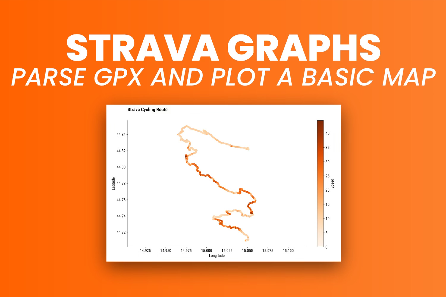
Remember to put longitude on the x-axis and latitude on the y-axis. Optionally, you can color the individual markers with another dataset column, such as speed in km/h:
plt.figure(figsize=(14, 8))
scatter = plt.scatter(df["longitude"], df["latitude"], cmap="Oranges", c=df["speed_kmh"], s=25)
plt.colorbar(scatter, label="Speed")

plt.title("Strava Cycling Route", loc="left", fontdict={"weight": "bold"}, y=1.06)
plt.xlabel("Longitude")
plt.ylabel("Latitude")
plt.axis("equal")
plt.show()
The route looks identical to the one in the first image, but keep in mind that I’ve removed the first and last 1000 points to mask the start/end points.
The only problem is that there’s no map behind it. In the following article, we’ll solve this issue by swapping the visualization library from Matplotlib to Plotly.
Wrapping up
To conclude, Python is your one-stop shop for analyzing and visualizing GPX files. You can dive much deeper into analytics than with applications such as Strava, and that’s just what you’ll build throughout the series.
Expect to build (and improve) the existing Strava charts, create new ones, and tie everything together into an interactive dashboard.